Single-Phase Capacitor-Input Rectifier

Based on: Ivo Barbi, Power Electronics, Chapter 10 — Rectifiers with Pure Capacitive Filter
Application: Complete theoretical and computational basis used in RectifierAbacos for capacitor sizing, current estimation, and harmonic analysis.

🔗 GitHub repository: Link

---

1. Introduction

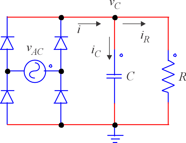
The single-phase full-wave rectifier with a capacitive filter is one of the most common topologies in low-power DC supplies.
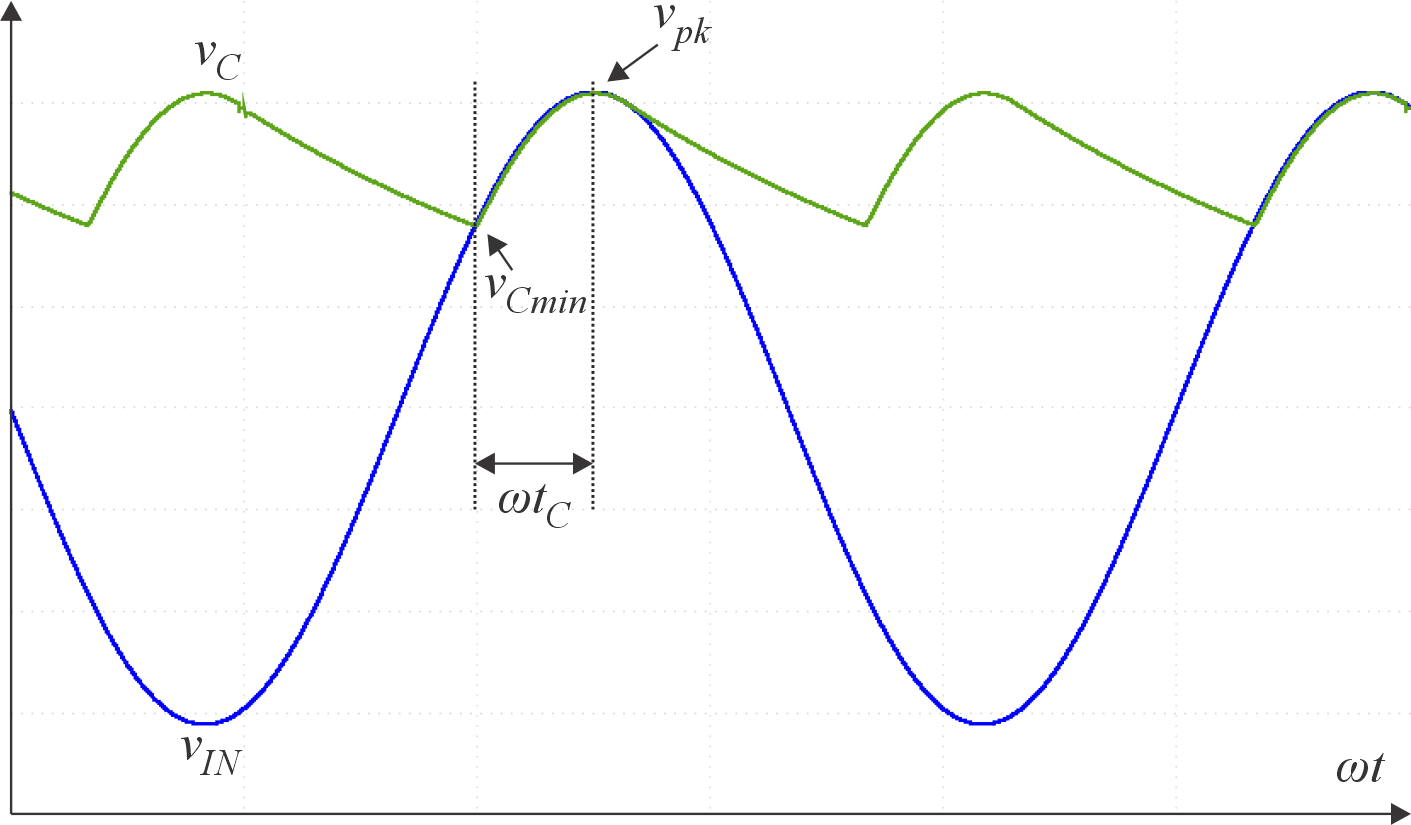
The capacitor charges during a short conduction interval when the input voltage exceeds the capacitor voltage, and discharges through the load during the remainder of the period.

Barbi’s analytical model describes the behavior of this circuit using normalized parameters that eliminate dependence on absolute voltage, resistance, and frequency values:

$$
x = \frac{V_{C\min}}{V_{pk}}, \qquad Y = \omega RC
$$

These relations define all subsequent analytical and numerical calculations implemented in RectifierAbacos.

---

2. Energy Balance and Capacitor Sizing(10.70)

The capacitor energy balance defines its value as a function of output power and ripple voltage.

$$
C = \frac{P_{out}}{f (V_{pk}^2 – V_{C\min}^2)}
$$

The conduction begins when the source voltage equals the capacitor voltage:

$$
V_{C\min} = V_{pk} \cos(\omega t_c)
$$

and the conduction time per half-cycle is:

$$
t_c = \frac{\arccos(V_{C\min}/V_{pk})}{2\pi f}
$$

The peak current in the capacitor (and through the diodes) during conduction is:

$$
I_{pk} = \frac{C (V_{pk} – V_{C\min})}{t_c}
$$

These expressions form the basis for capacitor sizing and component current stress estimation.

---

3. Abacus Relation — ωRC as a Function of V_Cmin/V_pk

The relation between $\omega RC$ and the voltage ratio $V_{C\min}/V_{pk}$ defines the fundamental abacus used in capacitor design.

(10.69)
$$
\omega C R (1 – \cos\alpha)
– \frac{\beta \cos\beta}{2}
– \omega C R \cos\beta
\left[ 1 – e^{\frac{(\alpha + \beta – \pi)}{\omega RC}} \right] = 0
$$

$$
\alpha = \frac{\pi}{2} – \sin^{-1}\left(\frac{V_{C\min}}{V_{pk}}\right)
$$

$$
\beta = \frac{\pi}{2} + \tan^{-1}(-\omega RC)
$$

These equations are solved numerically to produce the characteristic curve:

$$
\omega RC = f\left(\frac{V_{C\min}}{V_{pk}}\right)
$$

This curve represents the dimensionless capacitor sizing abacus in RectifierAbacos.

---

4. Average and RMS Currents

The instantaneous current is highly distorted.
For design purposes, Barbi provides expressions for the RMS and average values that define the electrical stresses of the components.

Capacitor RMS current:
$$
I_{C,ef} = I_{pk}\sqrt{2 t_c f – (2 t_c f)^2}
$$

Diode average and RMS currents:
$$
I_{D,avg} = \frac{P_{out}}{2 V_{C\min}}, \qquad
I_{D,ef} = I_{pk}\sqrt{\frac{t_c}{T}}
$$

Load average current:
$$
I_{L,avg} = \frac{P_{out}}{V_{C\min}}
$$

---

5. RMS Current in the Capacitor — Numerical Evaluation

The RMS current can be precisely obtained from the instantaneous current expressions for conduction and discharge intervals.

During conduction:
$$
i_{C1}(\theta) = \omega C V_{pk} \cos\theta
$$

During discharge:
$$
i_{C2}(\theta) = \frac{V_{pk}}{R} \cos\beta \; e^{\frac{\theta – \theta_2}{\omega RC}}
$$

RMS components:
$$
i_{C1,ef}^2 = \frac{1}{\pi}\int_{\theta_3}^{\theta_2}
\left( \frac{\omega RC V_{pk}}{R}\cos\theta \right)^2 d\theta
$$

$$
i_{C2,ef}^2 = \frac{1}{\pi}\int_0^{\theta_1 – \theta_2}
\left( \frac{V_{pk}}{R}\cos\beta \right)^2 e^{\frac{2\theta}{\omega RC}} d\theta
$$

Angle limits:
$$
\theta_1 = \pi + \sin^{-1}\left(\frac{V_{C\min}}{V_{pk}}\right),\quad
\theta_2 = \pi + \tan^{-1}(-\omega RC),\quad
\theta_3 = \sin^{-1}\left(\frac{V_{C\min}}{V_{pk}}\right)
$$

Total RMS capacitor current:
$$
I_{C,ef} = \sqrt{i_{C1,ef}^2 + i_{C2,ef}^2}
$$

---

6. Harmonic and Power-Quality Analysis

Expanding the input current into its Fourier series allows the analysis of harmonic distortion and power factor.
Only odd harmonics are present due to the half-wave symmetry.

Instantaneous current during conduction:
$$
i_1(\theta) = \omega C V_p \cos\theta + \frac{V_p}{R}\sin\theta
$$

Fourier coefficients:
$$
a_n = \frac{\pi}{2}\left[ \omega C V_p \int_{\theta_3}^{\theta_2}\cos\theta\cos(n\theta)d\theta +
\frac{V_p}{R}\int_{\theta_3}^{\theta_2}\sin\theta\cos(n\theta)d\theta \right]
$$

$$
b_n = \frac{\pi}{2}\left[ \omega C V_p \int_{\theta_3}^{\theta_2}\cos\theta\sin(n\theta)d\theta +
\frac{V_p}{R}\int_{\theta_3}^{\theta_2}\sin\theta\sin(n\theta)d\theta \right]
$$

Normalized coefficients:
$$
y = \omega C R,\quad
\bar{a}_n = y(A_1 + A_2),\quad
\bar{b}_n = y(B_1 + B_2),\quad
\bar{c}_n = \sqrt{\bar{a}_n^2 + \bar{b}_n^2}
$$

Derived quantities:
$$
\mathrm{THD} = \sqrt{\sum_{n=3,5,7,\dots}\left(\frac{I_n}{I_1}\right)^2},\quad
\phi_1 = \arctan\left(\frac{b_1}{a_1}\right),\quad
\mathrm{PF} = \cos\phi_1\,\frac{I_1}{I_{ef}}
$$

---

Three-Phase Capacitor-Input Rectifier

1. Introduction

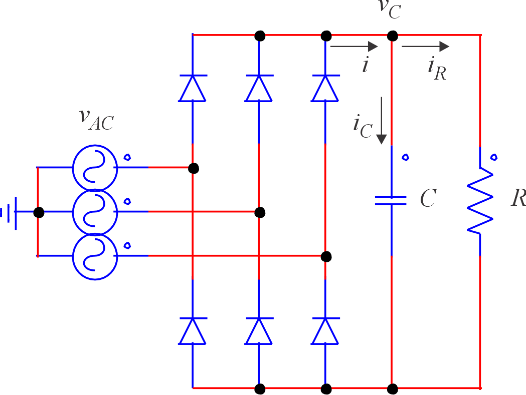
The three-phase full-wave rectifier with a capacitive output filter is widely employed in high-power DC link applications, such as DC bus supplies, UPS systems, and industrial drives. The capacitor smooths the output voltage, while the charging pulses occur at six times the line frequency (6f), resulting in smaller ripple and lower current stress than in the single-phase case.

---

2. Energy Balance and Capacitor Sizing

The capacitor value is determined by the energy balance between charge and discharge intervals. The voltage ripple at the DC output depends on the discharge time between consecutive conduction pulses of the rectifier.

$$ C = \frac{I_{dc}}{6f(V_{pk} – V_{C\min})} $$

Alternatively, in terms of output power and voltage:

$$ C = \frac{P_{out}}{3V_{C\min}(V_{pk} – V_{C\min})6f} $$

Since the charging pulses repeat every 60°, the voltage ripple is significantly smaller than in the single-phase rectifier for the same load current and capacitance value.

---

3. Conduction Angle and Peak Current

The conduction starts when the instantaneous phase-to-phase voltage equals the capacitor voltage. The conduction angle per phase is given by:

$$ \theta_c = \arccos\left(\frac{V_{C\min}}{V_{LL,pk}}\right) $$

Peak diode current:

$$ I_{pk} = \frac{C(V_{LL,pk} – V_{C\min})}{t_c} $$

where $V_{LL,pk}$ is the line-to-line voltage peak and $t_c$ is the conduction duration corresponding to $\theta_c$.

---

4. Capacitor RMS and Diode Currents

During each charging pulse, two diodes conduct simultaneously, and the capacitor current waveform consists of six narrow pulses per cycle. The RMS and average currents can be approximated by analytical relations derived by Barbi.

Capacitor RMS current:
$$ I_{C,ef} = \sqrt{6} I_{pk}\sqrt{\frac{t_c}{T}} $$

Diode RMS current:
$$ I_{D,ef} = I_{pk}\sqrt{\frac{t_c}{T}} $$

Load average current:
$$ I_{L,avg} = \frac{P_{out}}{V_{C\min}} $$

---

5. Abacus Relation — ωRC as a Function of V_Cmin/V_pk

The dimensionless product $\omega RC$ can be determined using the analytical relation provided by Barbi for the three-phase case. The following equations (adapted from Eqs. 10.88 – 10.90) define the abacus curve implemented in RectifierAbacos.

(10.88)
$$ \omega RC(1 – \cos\alpha) – \frac{\beta \cos\beta}{3} – \omega RC\cos\beta \left[ 1 – e^{\frac{(\alpha + \beta – \pi/3)}{\omega RC}} \right] = 0 $$

(10.89)
$$ \alpha = \frac{\pi}{6} – \sin^{-1}\left(\frac{V_{C\min}}{V_{LL,pk}}\right) $$

(10.90)
$$ \beta = \frac{\pi}{6} + \tan^{-1}(-\omega RC) $$

Solving these numerically gives the curve $\omega RC = f(V_{C\min}/V_{LL,pk})$, which is the main abacus for capacitor selection in three-phase rectifiers.

---

6. Harmonic and Power-Quality Analysis

The line current of a three-phase, six-pulse rectifier with a capacitive output filter presents half-wave symmetry, as described by:

$$
f(\theta) = f(\theta – \pi)
$$

Therefore, only odd harmonics appear in the Fourier expansion of the input current.
The instantaneous current in phase *a* and phase *b* are given by:

$$
i_a(\theta) = \omega C V_p \cos(\theta) + \frac{V_p}{R}\sin(\theta)
$$

$$
i_b(\theta) = \omega C V_p \cos(\theta – \tfrac{\pi}{3}) + \frac{V_p}{R}\sin(\theta – \tfrac{\pi}{3})
$$

The capacitor current adds to the resistive component to form the total line current.
Outside these conduction intervals, the line current is zero.
The Fourier coefficients for the sine and cosine terms are defined as:

$$
a_n = \frac{2}{\pi}
\left[
\int_{\theta_3}^{\theta_2} i_a(\theta)\cos(n\theta)\,d\theta +
\int_{\theta_3 + \pi/3}^{\theta_2 + \pi/3} i_b(\theta)\cos(n\theta)\,d\theta
\right]
$$

$$
b_n = \frac{2}{\pi}
\left[
\int_{\theta_3}^{\theta_2} i_a(\theta)\sin(n\theta)\,d\theta +
\int_{\theta_3 + \pi/3}^{\theta_2 + \pi/3} i_b(\theta)\sin(n\theta)\,d\theta
\right]
$$

For normalization and graphical representation of harmonic amplitudes, Barbi adopts the parametrization:

$$
\frac{\pi R}{2V_p}a_n = \bar{a}_n, \qquad
\frac{\pi R}{2V_p}b_n = \bar{b}_n
$$

Consequently, the amplitude of the normalized harmonic component is expressed as:

$$
\bar{c}_n = \sqrt{\bar{a}_n^2 + \bar{b}_n^2}
$$